
Residential Property Value Prediction
Multi-market residential property value prediction using 10,659 transactions across 50 U.S. college-town housing markets, with regression, Random Forest, Bagging, Gradient Boosting, cross-validation, and feature-importance analysis.
Project Overview
Rebuilt and expanded an earlier University of North Texas residential property valuation project to use the complete dataset of 10,659 residential transactions across 50 U.S. college-town housing markets.
The original coursework analyzed only 211 transactions associated with Iowa State University in Ames, Iowa. The expanded portfolio version revisits the same underlying dataset with a broader analytical question:
How well can residential property values be predicted when property characteristics and major differences between local housing markets are modeled together?
The rebuilt analysis uses Python to compare multiple linear-regression specifications with Bagging, Random Forest, and Gradient Boosting models while preserving all 10,659 observations.
Project Objectives
The expanded analysis focused on:
- replacing the original single-market sample with the complete 10,659-transaction dataset;
- evaluating residential values across 50 distinct housing markets;
- identifying and retaining legitimate high-value and large-property observations rather than automatically removing them as outliers;
- reducing extreme skew through justified logarithmic transformations;
- explicitly controlling for housing-market location;
- comparing interpretable regression models with nonlinear ensemble methods;
- evaluating models using RMSE, MAE, MAPE, R², cross-validation, and held-out testing;
- identifying the strongest predictors of residential property value; and
- producing a reproducible, portfolio-ready analytical workflow.
Dataset
The source workbook contains residential transactions associated with 50 universities and 50 corresponding college-town housing markets.
The complete analytical dataset contains:
- 10,659 residential transactions
- 50 towns
- 50 universities
- 3 property types
- no missing values in the modeled variables; and
- no duplicate records.
Because each town corresponded one-to-one with a university in the source data, Town was used as the geographic market variable rather than including both fields and creating redundant location controls.
Core Variables
The primary property characteristics were:
BedsBathsSqft_homeSqft_lotTypeAgeTown
The prediction target was:
Sale_amount
Property age was calculated at the time of sale, rather than using the property’s age at the current date.
Data Preparation and Outlier Review
Exploratory analysis showed substantial right skew in several variables.
Observed skewness included approximately:
Sale_amount: 5.87Sqft_home: 53.8Sqft_lot: 19.2
The full dataset also contained unusually large residential properties, including a multifamily transaction with more than 140,000 square feet.
Rather than automatically deleting these records, the analysis inspected them individually and retained them when the surrounding fields were internally consistent.
Logarithmic transformations were therefore created for:
Sale_amountSqft_homeSqft_lot
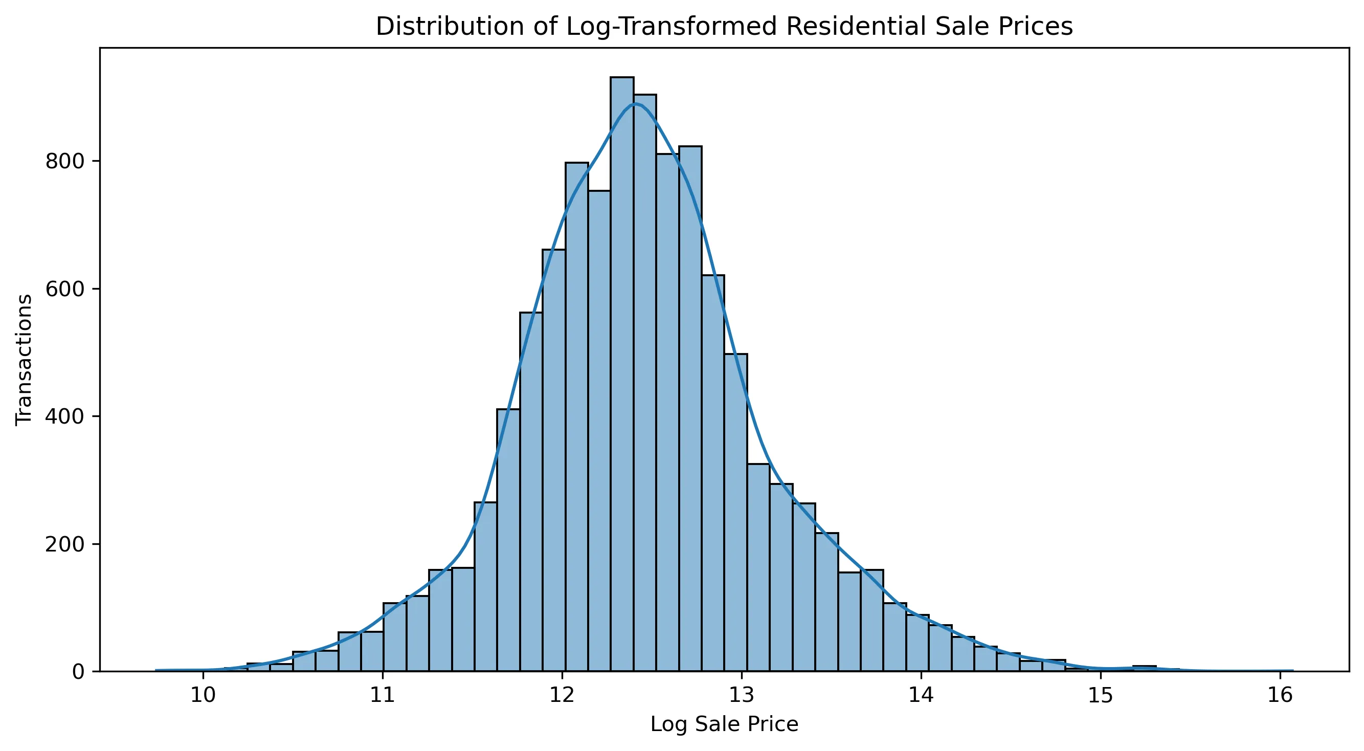
The transformation reduced sale-price skew from approximately 5.87 to 0.36 and home-square-footage skew from approximately 53.8 to 0.36, allowing the analysis to preserve the complete dataset while limiting the influence of extremely large observations.
Sale Price Distribution
The raw residential sale-price distribution was heavily right-skewed because a relatively small number of high-value properties extended far beyond the center of the market.
A logarithmic transformation produced a substantially more balanced distribution and became the basis of the strongest linear-regression specification.
Regression Modeling
Three Ordinary Least Squares specifications were evaluated.
Model 1 — Raw-Dollar Baseline
The first model predicted sale price directly using the original property measurements plus market and property-type controls.
Sale_amount ~ Beds + Baths + Sqft_home + Sqft_lot + C(Type) + C(Town) + Age
The model produced an in-sample R² of approximately 0.720, but residual analysis showed substantial heteroskedasticity as property values increased.
Model 2 — Raw-Dollar Model with Transformed Property Size
The second specification retained sale price in dollars while transforming the highly skewed square-footage predictors.
Sale_amount ~ Baths + Log_Sqft_home + Log_Sqft_lot + C(Type) + C(Town) + Age
Its in-sample R² declined to approximately 0.696, and the residual pattern remained strongly heteroskedastic.
Model 3 — Log-Transformed Sale Value
The third model transformed both the target and major size predictors.
Log_Sale_amount ~ Baths + Log_Sqft_home + Log_Sqft_lot + C(Type) + C(Town) + Age
This specification produced:
- R²: approximately 0.777
- Adjusted R²: approximately 0.776
- substantially improved residual behavior; and
- a more balanced treatment of properties across different price levels.
HC3 heteroskedasticity-robust standard errors were also evaluated for the regression specifications.
Regression Cross-Validation
The three regression models were compared using 10-fold cross-validation with shuffled, reproducible folds.
Because Model 3 predicts log sale values, its predictions were converted back into actual dollars using a Duan smearing correction before calculating prediction errors.
| Regression Model | RMSE | MAE | MAPE |
|---|---|---|---|
| Model 1 — Raw-Dollar Baseline | $197,660.95 | $91,374.85 | 32.25% |
| Model 2 — Transformed Property Size | $190,049.98 | $102,127.61 | 39.76% |
| Model 3 — Log Sale Value | $599,415.53 | $93,723.30 | 27.52% |
The cross-validation results illustrate an important modeling trade-off.
Model 1 produced the lowest typical absolute-dollar error, Model 2 produced the lowest RMSE, and Model 3 produced the lowest percentage error.
Model 3 therefore improved fit and relative prediction consistency across the broader housing market, but very high-value transactions created large retransformed dollar errors.
Ensemble Tree Models
The nonlinear modeling stage evaluated three ensemble approaches:
- Bagging Regressor
- Random Forest Regressor
- Gradient Boosting Regressor
Categorical Town and Type variables were one-hot encoded, producing a 58-column predictor matrix.
The complete dataset was then divided into:
- 8,527 training observations — 80%
- 2,132 held-out test observations — 20%
The same held-out test set was used for all three ensemble models.
Hyperparameters were tuned using GridSearchCV on the training data only.
Bagging Regressor
The best Bagging configuration used:
- 200 estimators
- unrestricted tree depth
- 80% maximum sample size
Random Forest
The strongest Random Forest configuration used:
- 400 estimators
- unrestricted maximum depth
- square-root feature sampling
Gradient Boosting
The strongest Gradient Boosting configuration used:
- 200 estimators
- learning rate of 0.10
- maximum tree depth of 3
Ensemble Model Performance
| Model | RMSE | MAE | MAPE | R² |
|---|---|---|---|---|
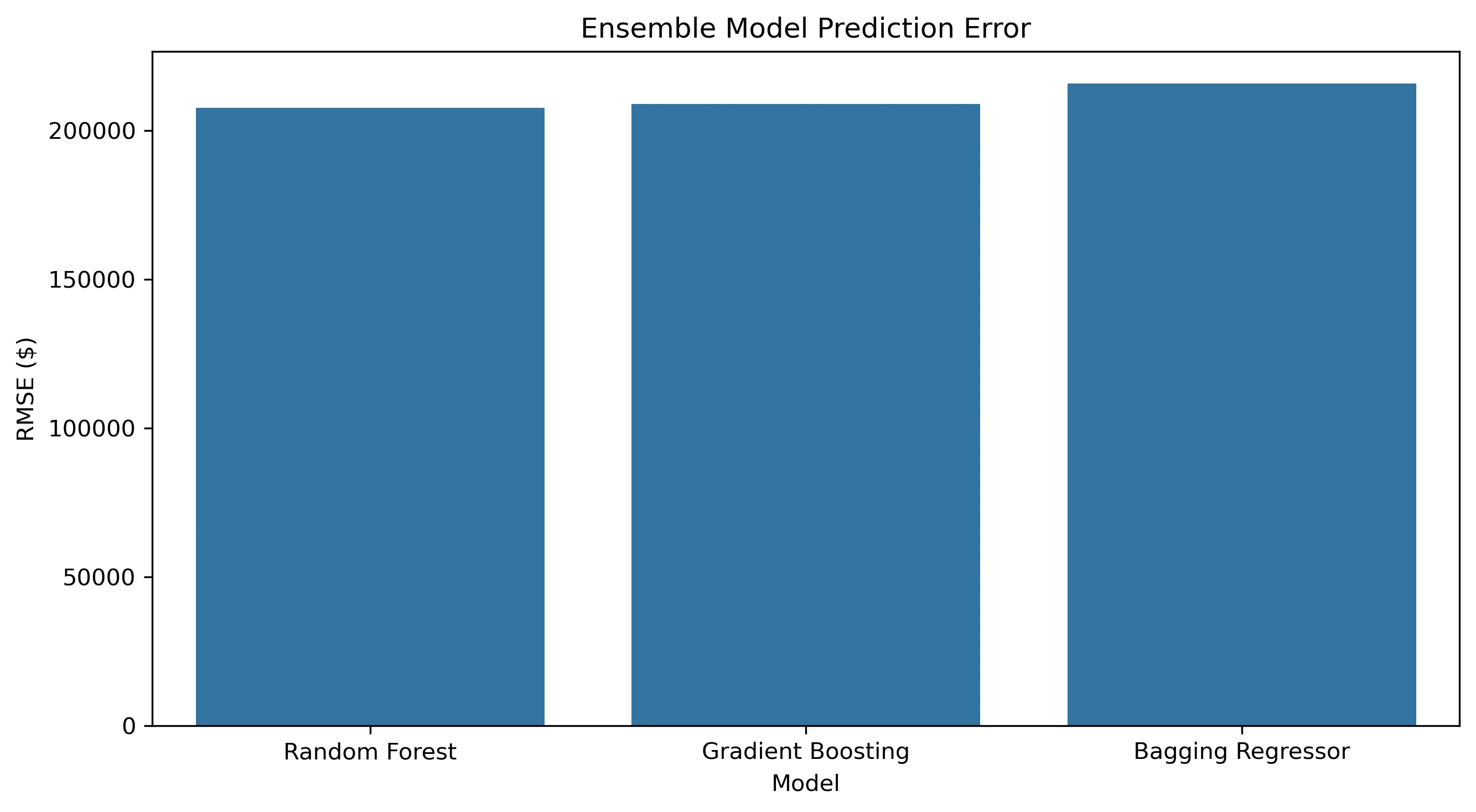
| Random Forest | $207,602.31 | $75,651.69 | 27.09% | 0.6926 |
| Gradient Boosting | $209,040.04 | $81,917.90 | 29.50% | 0.6884 |
| Bagging Regressor | $215,824.95 | $78,242.53 | 26.92% | 0.6678 |
Random Forest provided the strongest overall held-out test performance.
It produced the:
- lowest RMSE;
- lowest MAE; and
- highest R².
Bagging produced a slightly lower MAPE, outperforming Random Forest by only 0.17 percentage points on that metric.
Random Forest was therefore selected as the strongest overall ensemble model rather than because it dominated every possible measure.
What Drives Residential Property Value?
The expanded model produced a materially different insight from the original Ames-only analysis.
After the 50 town indicators were aggregated back into a single market-location feature group, Random Forest importance was approximately:
| Predictor Group | Random Forest Importance |
|---|---|
| Town / Housing Market | 45.48% |
| Home Square Footage | 19.47% |
| Bathrooms | 11.69% |
| Lot Square Footage | 8.71% |
| Property Age | 8.21% |
| Bedrooms | 4.89% |
| Property Type | 1.55% |
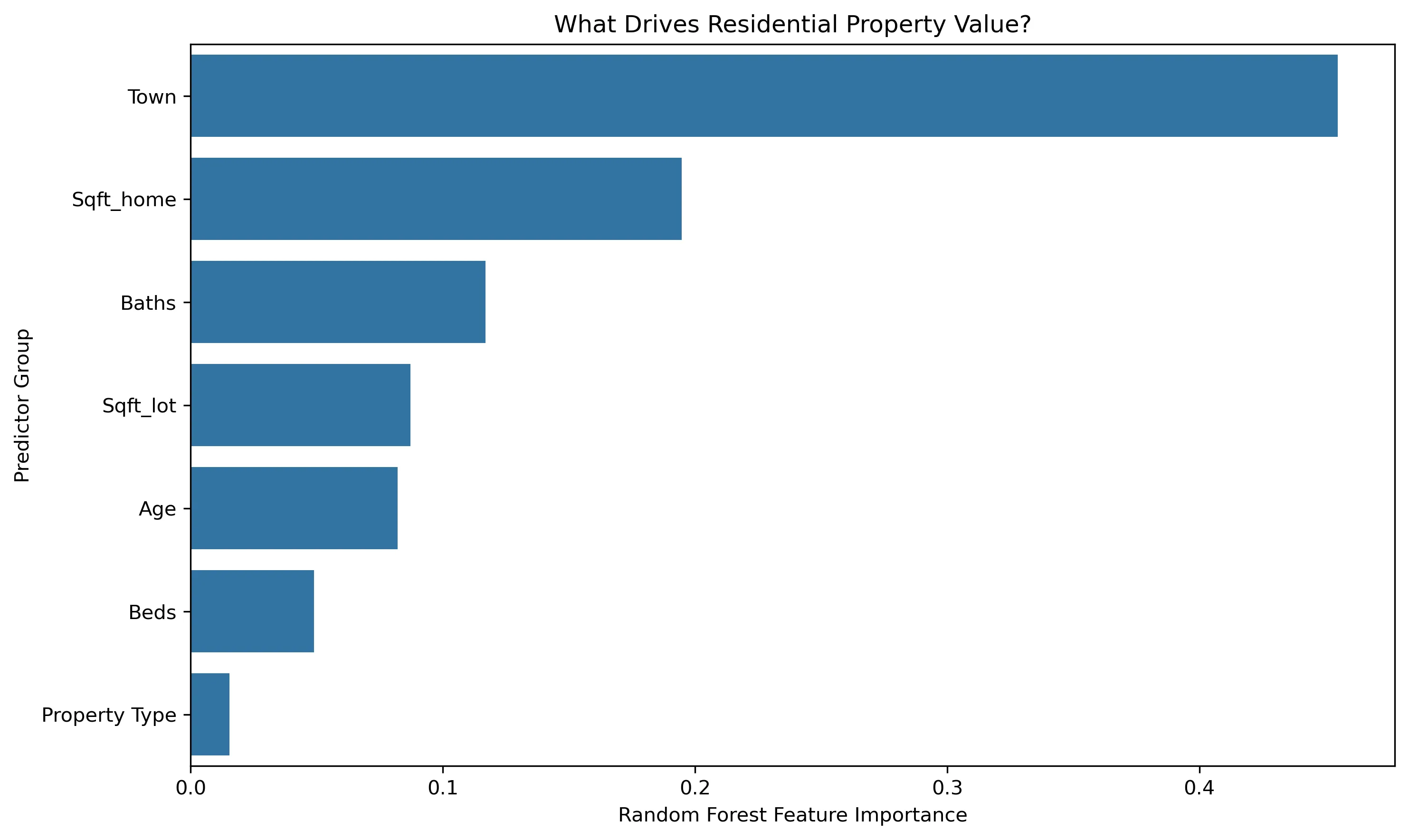
The result shows that location was collectively the dominant source of predictive information, followed by home size.
Bathrooms, lot size, property age, and bedroom count contributed additional information once differences between local housing markets were represented explicitly.
These percentages are model-based feature importances, not causal effects. They describe how the trained Random Forest used the available predictors; they should not be interpreted as percentages of a property’s price caused by each characteristic.
Key Findings
The expanded analysis produced four primary findings.
1. Housing markets matter substantially.
Town-level market indicators collectively represented approximately 45% of Random Forest feature importance.
2. Home size remained the strongest individual physical predictor.
Home square footage accounted for approximately 19% of overall Random Forest feature importance.
3. Log transformation substantially improved the linear-model specification.
The log-price regression achieved an R² of approximately 0.78 and substantially improved residual behavior compared with the raw-dollar specifications.
4. Model selection depends on the error being optimized.
No model universally dominated every metric. Random Forest provided the strongest overall held-out ensemble performance, while other specifications performed better on individual error measures.
Analytical Limitations
The expanded project substantially improves on the original single-market analysis, but it is not a production appraisal system.
Important limitations include:
- the dataset is concentrated in college-town housing markets rather than representing all U.S. residential transactions;
- important valuation variables such as neighborhood-level characteristics, renovation quality, school districts, interest rates, taxes, and detailed property condition are not included;
- one-hot encoded town indicators represent observed market differences but do not explain the economic causes of those differences;
- high-value and unusually large properties create substantial absolute-dollar prediction errors;
- Random Forest feature importance is predictive rather than causal; and
- evaluation results depend on the specific training/test and cross-validation procedures used.
The model should therefore be interpreted as an analytical demonstration of residential-value prediction across heterogeneous markets rather than as a professional appraisal or automated valuation product.
Reconstruction and Expansion Improvements
The portfolio release extends the original academic project substantially.
Improvements include:
- expansion from 211 Ames observations to all 10,659 transactions;
- expansion from one housing market to 50 college-town markets;
- correction of property age to reflect age at time of sale;
- retention and inspection of extreme observations rather than arbitrary deletion;
- logarithmic transformation of heavily skewed variables;
- explicit market-location controls;
- preservation of all three property types rather than binary simplification;
- reproducible 10-fold regression cross-validation;
- Duan smearing correction for retransformed log predictions;
- proper implementation of a Bagging Regressor;
- tuned Random Forest and Gradient Boosting models;
- consistent 80/20 held-out testing for ensemble comparison;
- grouped feature-importance analysis;
- repository-relative data paths;
- portfolio-ready visualizations; and
- expanded technical documentation and limitations.
Skills Demonstrated
- Python
- Jupyter Notebook
- pandas
- NumPy
- statsmodels
- scikit-learn
- Exploratory Data Analysis
- Data cleaning and preprocessing
- Feature engineering
- Log transformations
- Linear regression
- Heteroskedasticity-robust inference
- Bagging
- Random Forest
- Gradient Boosting
- One-hot encoding
- Cross-validation
- Hyperparameter tuning
- GridSearchCV
- Model evaluation
- RMSE / MAE / MAPE / R²
- Feature importance analysis
- Data visualization
- Git / GitHub version control
- Technical documentation
- Reproducible analytical workflows
Project Status
Expanded portfolio analysis complete.
The project now includes:
- the full 10,659-transaction analytical dataset;
- a reconstructed and expanded Python notebook;
- three regression specifications;
- three ensemble models;
- cross-validation and held-out test evaluation;
- feature-importance analysis;
- portfolio visualizations;
- documented analytical limitations; and
- a dedicated public GitHub repository.
Project Provenance
This project originated as a group academic project for ADTA 4230 — Data Analytics and Computational Statistics 2 at the University of North Texas.
The original academic analysis focused on the Iowa State University / Ames subset of the source workbook.
The subsequent reconstruction and portfolio expansion—including use of the complete 10,659-transaction dataset, multi-market modeling, revised preprocessing, model validation, repository development, technical documentation, and public-facing presentation—were completed as part of the Portfolio Project & Analytics Development initiative.
Technical Evidence
The public project repository contains the expanded analysis notebook, regression and ensemble-model workflows, portfolio visualizations, dependency documentation, and supporting technical notes.